Classifying clothing: the quest for the non-orientable tank top.
January 22, 2007 personal
When I walk down the street, I create patterns in how I walk, often by controlling my stride length so I will step on cracks every third sidewalk square, or whatnot. If I were a true master, my stride length would be incommensurable with respect to the sidewalk length–surely this was the problem that forced irrationalities upon the Greeks…
Anyway, I was also happy to realize (at a recent retreat) that clothing is nicely categorized by how many disks must be removed from a sphere to produce the particular clothing item. For some examples, consider:
- A sock or a hat is a sphere minus a disk.
- A headband (or tube top) is a sphere minus two disks.
- Jeans are a sphere minus three disks (the fabled “pair of pants”).
- A shirt is a sphere minus four disks (the “lantern”).
- A bathing suit is a sphere minus five disks.
- A fingerless glove might be a sphere minus six disks.
- Two fingerless gloves connected by a band is a sphere minus 11 disks.
Another lovely example is that of some scarves, which are a projective plane minus a disk (i.e., a Mobius strip), and therefore sit flat against one’s neck. I would be very interested in owning more non-orientable clothing (someone, somewhere, must own a non-orientable tank top–though perhaps that mythical object would be too annoying to be allowed to exist).
Corrugated coffee cup holders.
January 17, 2007 personal
I’ve been (not surprisingly) drinking quite a bit of coffee lately, and I’ve noticed that many corregated coffee cup holders include a bit of loose glue. At first, I thought this was a mistake, an oversight in the perfection of the coffee cup holder design.
On the contrary, that bit of excess glue melts when the hot coffee is poured into the cup, adhering the corregated holder to the cup–brilliant!
Estimating the speed of the plane.
January 16, 2007 physics
I’m sometimes bored while flying, and I like looking out the window (though if I can, I usually pick aisle seats so I can exit more quickly).
I realized something rather amusing. I closed one eye, and held two fingers about an inch apart and a foot away from my open eye. Then, I timed how long it took an object on the ground to move from the one finger to the other finger an inch away; it took about ten seconds.
Let be the distance in feet from my eye to that point on the ground. By similar triangles, moving an inch when one foot away from my eye means moving inches on the ground. The distance from my eye to the ground is (wild guess!) 60,000 feet, so the point on the ground actually moved 60,000 inches, or 5000 feet, about a mile. Moving a mile in ten seconds is moving six miles per minute, or 360 miles per hour.
I seem to recall that 450 mph is actually how fast a commercial jet might go, so at least I’m within an order of magnitude. Now 450 miles per hour would have been 39,600 feet per minute, or 6600 feet in ten seconds, or 79,200 inches in ten seconds, so maybe I should’ve estimated 80,000 feet to the ground. But there are so many other sources of error in this technique…
Are there other fun things to estimate when trapped on a plane?
Most numbers are boring, asymptotically speaking.
December 10, 2006 personal
Let be the number of Google hits for the integer . Then is about 100 million, and , that is, the number of hits for a number twice as big, is about 40 million, a bit less than half as big. Doubling the input continues to halve the output: is about 20 million (half again!), and is about 8 million, and is about 4 million.
There are about half as many pages talking about numbers that are twice as big. This is an example of a power law, and indeed, a log-log plot of looks linear to my blurry vision:
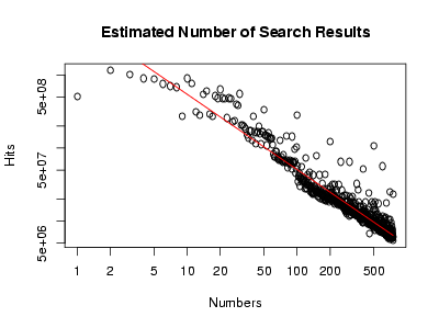
Doing a linear regression in R gives the red line, or in symbols, Rather humorously, this means that . In the end, this is not so surprising: Zipf’s law says that, in a corpus of naturally occuring text, the frequency of a word is inversely proportional to its rank; here, we have a similar phenomenon at work: roughly, the popularity of a number is inversely proportional to its size.
In other words, while the number of integers expressible with fewer than bits grows exponentially in , the number of pages discussing integers expressible with fewer than bits grows linearly in ; being silly, I’d say that this is an asymptotic version of the claim that most large numbers are uninteresting. After all, popular numbers have a lot of fan sites.
On the Popularity of Certain Numbers.
December 3, 2006 personal
I searched for each number between 1 and 500 on Google, and recorded the (estimated) number of hits. I’m not aware of anyone having done this before; in any case, I made a chart:

Click on the above chart to see a bigger version. You can also look more closely at the first hundred numbers, or look at the above data with a log scale on the y-axis.
I have some observations and questions:
- There’s some periodicity in the above data (every 5, every 10, every 100).
- Can you explain how quickly the distribution falls off (is it exponentially decaying, for instance)?
- The most popular numbers are, in decreasing order of popularity: 2, 3, 10, 4, 5, 11, 6, 7, 8, 20, 15, 30, 14, 18, 1, 24, 21, 19, 25, 22, 28, 29, 50, and so on.
- The most popular numbers ending in 0 are, in decreasing order of popularity and having been divided by ten: 1, 2, 3, 5, 10, 4, 8, 9, 7, 20, 6, 50, 15, 12, 30, 25, 11, 40, 13, 18, 16, 14, and so on. Is the distribution of numbers ending in 0 related to the distribution of all numbers?
- Are certain families of numbers more popular? Are prime numbers or square numbers particularly popular?
You can download my comma-separated data file if you would like to play with the data yourself. Note, however, that I got this data from Google’s SOAP interface, which, for reasons I don’t understand, doesn’t give the same number of “estimated hits” as the web page interface.
Growth series.
November 30, 2006 general
In seminar today, Okun pointed out the following interesting observation; for any finitely generated group , you can define its growth series , where is the length of the shortest word for . The first observation is that is often a rational function, in which case makes sense. The second observation is that is “often” equal to . This is an example of weighted cohomology.
Grigorchuk’s group (and generally any group with intermediate (i.e., subexponential but not polynomial) growth) does not have a rational growth function; the coefficients in a power series for a rational function grow either polynomially or exponentially. This observation appears in [1]. More significantly, this paper constructs groups which, being nilpotent, have polynomial growth, but nonetheless have generating sets for which that the corresponding growth series is not rational.
[1] M. Stoll, Rational and transcendental growth series for the higher Heisenberg groups, Invent. Math. 126 (1996) 85–109.
Constructing a Lie group from a Lie algebra.
November 30, 2006 mathematics
Cartan proved that every finite-dimensional real Lie algebra Error:LaTeX failed:
This is pdfTeX, Version 3.141592653-2.6-1.40.22 (TeX Live 2021/nixos.org) (preloaded format=latex)
 restricted \write18 enabled.
entering extended mode
(./working.tex
LaTeX2e <2021-11-15> patch level 1
L3 programming layer <2022-02-24>

(/nix/store/pibhz89i08877bwjc13mmq7b3kaqkmhi-texlive-combined-full-2021-final/s
hare/texmf/tex/latex/base/article.cls
Document Class: article 2021/10/04 v1.4n Standard LaTeX document class

(/nix/store/pibhz89i08877bwjc13mmq7b3kaqkmhi-texlive-combined-full-2021-final/s
hare/texmf/tex/latex/base/size12.clo))
(/nix/store/pibhz89i08877bwjc13mmq7b3kaqkmhi-texlive-combined-full-2021-final/s
hare/texmf/tex/latex/preview/preview.sty
(/nix/store/pibhz89i08877bwjc13mmq7b3kaqkmhi-texlive-combined-full-2021-final/s
hare/texmf/tex/generic/luatex85/luatex85.sty)
(/nix/store/pibhz89i08877bwjc13mmq7b3kaqkmhi-texlive-combined-full-2021-final/s
hare/texmf/tex/latex/preview/prtightpage.def))
(/nix/store/pibhz89i08877bwjc13mmq7b3kaqkmhi-texlive-combined-full-2021-final/s
hare/texmf/tex/latex/amsmath/amsmath.sty
For additional information on amsmath, use the `?' option.

(/nix/store/pibhz89i08877bwjc13mmq7b3kaqkmhi-texlive-combined-full-2021-final/s
hare/texmf/tex/latex/amsmath/amstext.sty
(/nix/store/pibhz89i08877bwjc13mmq7b3kaqkmhi-texlive-combined-full-2021-final/s
hare/texmf/tex/latex/amsmath/amsgen.sty))
(/nix/store/pibhz89i08877bwjc13mmq7b3kaqkmhi-texlive-combined-full-2021-final/s
hare/texmf/tex/latex/amsmath/amsbsy.sty)
(/nix/store/pibhz89i08877bwjc13mmq7b3kaqkmhi-texlive-combined-full-2021-final/s
hare/texmf/tex/latex/amsmath/amsopn.sty))
(/nix/store/pibhz89i08877bwjc13mmq7b3kaqkmhi-texlive-combined-full-2021-final/s
hare/texmf/tex/latex/amsfonts/amsfonts.sty)
(/nix/store/pibhz89i08877bwjc13mmq7b3kaqkmhi-texlive-combined-full-2021-final/s
hare/texmf/tex/latex/base/fontenc.sty)
(/nix/store/pibhz89i08877bwjc13mmq7b3kaqkmhi-texlive-combined-full-2021-final/s
hare/texmf/tex/latex/lm/lmodern.sty)
(/nix/store/pibhz89i08877bwjc13mmq7b3kaqkmhi-texlive-combined-full-2021-final/s
hare/texmf/tex/latex/lm/t1lmr.fd)
(/nix/store/pibhz89i08877bwjc13mmq7b3kaqkmhi-texlive-combined-full-2021-final/s
hare/texmf/tex/latex/l3backend/l3backend-dvips.def)
No file working.aux.
Preview: Fontsize 12pt

(/nix/store/pibhz89i08877bwjc13mmq7b3kaqkmhi-texlive-combined-full-2021-final/s
hare/texmf/tex/latex/lm/ot1lmr.fd)
(/nix/store/pibhz89i08877bwjc13mmq7b3kaqkmhi-texlive-combined-full-2021-final/s
hare/texmf/tex/latex/lm/omllmm.fd)
(/nix/store/pibhz89i08877bwjc13mmq7b3kaqkmhi-texlive-combined-full-2021-final/s
hare/texmf/tex/latex/lm/omslmsy.fd)
(/nix/store/pibhz89i08877bwjc13mmq7b3kaqkmhi-texlive-combined-full-2021-final/s
hare/texmf/tex/latex/lm/omxlmex.fd)
(/nix/store/pibhz89i08877bwjc13mmq7b3kaqkmhi-texlive-combined-full-2021-final/s
hare/texmf/tex/latex/amsfonts/umsa.fd)
(/nix/store/pibhz89i08877bwjc13mmq7b3kaqkmhi-texlive-combined-full-2021-final/s
hare/texmf/tex/latex/amsfonts/umsb.fd)
! Undefined control sequence.
l.11 \germ
           g
Preview: Tightpage -32891 -32891 32891 32891
[1] (./working.aux) )
(see the transcript file for additional information)
Output written on working.dvi (1 page, 1620 bytes).
Transcript written on working.log.
comes from a connected, simply-connected Lie group . I hadn’t known the proof of this result (and apparently it is rather uglier than one might hope), but [1] gives a short proof of it, which I presented to the undergraduates in my Lie group seminar. I’ll sketch the proof now.
Theorem. For every Lie algebra , there is a simply-connected, connected Lie group having as its Lie algebra.
First, if , then the exponential map gives , and we define . It turns out is a Lie group, and is its Lie algebra.
If has no center, then is injective, so we have realized as a Lie subalgebra of endomorphisms of a vector space, and by the above, there is a Lie group with as its Lie algebra. Taking its universal cover proves the theorem in this case.
Now we induct on the dimension of the center . Let be a one-dimensional central subspace of , and construct a short exact sequence . But this central extension of by corresponds to a 2-cocycle .
Lemma. Let be the map which differentiates a (smooth!) -cocycle of the group cohomology of . The map is injective.
Consequently, we can find with . Since , by induction there is a Lie group having as its Lie algebra. We build the central extension of by using the cocycle , namely, , where and the operation is . Since , it turns out that the Lie algebra corresponding to is . We finish the proof by taking the universal cover .
[1] V.V. Gorbatsevich, Construction of a simply connected group with a given lie algebra, Uspekhi Mat. Nauk. 41 (1986) 177–178.
History of Static Electricity?
November 29, 2006 personal
What can be said about the history of static electricity? Did Greek science know about it? Any medieval experiments with static electricity?
It’s sort of interesting that people knew about magnetism and electricity for hundreds of years before finding many good uses for that knowledge (granted, compasses and potentially batteries for electroplating, but these things are trinkets in our modern world so dependent on electricity); in contrast, the span between radiation and harnessing nuclear power was much shorter (although maybe our modern uses of nuclear power will seem like mere trinkets compared to the awesome uses to come). I guess this isn’t surprising—eh, nothing I say is surprising!
And after listening to Sufjan Stevens’ “A Good Man is Hard to Find,” I read the short story with the same title. I find myself liking “Seven Swans” more and more, and the short story by Flannery O’Connor was quite interesting. The short story of the crane wife (which is used to good effect on the Decemberists new album of the same name) is quite beautiful, too.
And last night, while doing some mathematics, I was also listening to an audiobook (well, podcast) rendition of Plato’s Republic; I had forgotten the thing about the ring that turned people invisible! It’s funny enough that this gets picked up in the Lord of the Rings, but just the idea of such a ring is so provocative—where did the idea come from?
And earlier this week, I was reading about king David’s “mighty men” and about the beautiful Abishag. I find it amusing how the names of these people (e.g., Glaucon in The Republic or Abishag) get remembered, with fame far beyond their expectation, I’m sure.
Experiments in cooking.
November 28, 2006 personal
I tried making bread, but with significantly less flour than neccessary (and therefore, far more water than needed). The result was very much like cooked paste. It was pointed out to me that since the essence of bread is flour, trying to get by with less flour was undermining the very essence of bread (and I find such arguments very satisfying).
I also made baklava again, and that turned out much better than the first time (which involved the baklava burning).
Coxeter group visualization.
November 28, 2006 mathematics
Jenn is a fabulous program for visualizing the Cayley graphs of finite Coxeter groups. The pictures are absolutely beautiful (oh, symmetry!).