Google Trends plots the search volume (or some other measure? search percentage?) for a given phrase over time. It’s ridiculously fun!

As an example, let’s look at the number of times people search for the words hot and cold. I downloaded the CSV file offered by Google trends to make the following graph:

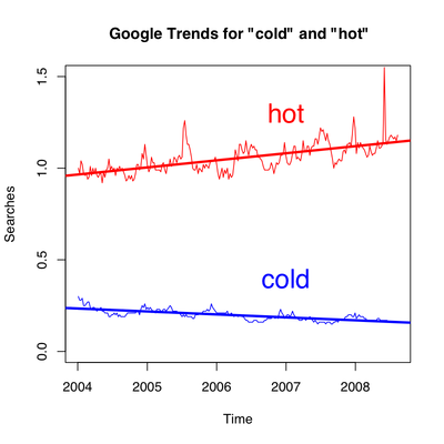
The thick red and blue lines are the linear regressions on the number of searches for hot and cold, respectively. Behold!—people are searching more often for hot lately, and less often as of late for cold! The search volume does seem to be related to the temperature: you might notice that the search volume for cold dips under the regression line during the summer, but exceeds it during the winter.

And so, global warming is being revealed in our search habits. Maybe I should’ve titled this post “Google warming.”

The Romans (among others!) wrote in wax with a stylus; the wax was embedded in boards, which were bound together in pairs. If a Roman were to place clay between these boards, could they make a copy of their wax tablet in the clay?

It strikes me as remarkable that coins were minted so long before books were printed—though I guess the motivation behind minting coins and printing books are rather different.

I gave a talk in the Farb and Friends Student Seminar (back in March!) on [1].

This is an awesome paper—well-worth a few words on every blog!

The construction is way easier than you might think. The ingredients:

• A model space with a map
• Any simplicial complex with a nondegenerate (edge-non-collapsing) map (if having a map to seems like a bother, note that the barycentric subdivision comes with a map to for free).

Let for a subcomplex of ; we think of this as decomposing into pieces resembling a simplex.

Now the construction is easy: replace each simplex in with a corresponding piece of . Or more formally, build the fiber product of and over ; this fiber product is denoted by in the paper. From this, we get a natural map .

The vague upshot is this: features of translate into features of , while nonetheless preserving features of . Here are a couple of examples of how assumptions on lead to consequence for .

• If is path-connected, and for each codimension 1 face of , we have Error:LaTeX failed:
  This is pdfTeX, Version 3.141592653-2.6-1.40.22 (TeX Live 2021/nixos.org) (preloaded format=latex) restricted \write18 enabled. entering extended mode (./working.tex LaTeX2e <2021-11-15> patch level 1 L3 programming layer <2022-02-24> (/nix/store/pibhz89i08877bwjc13mmq7b3kaqkmhi-texlive-combined-full-2021-final/s hare/texmf/tex/latex/base/article.cls Document Class: article 2021/10/04 v1.4n Standard LaTeX document class (/nix/store/pibhz89i08877bwjc13mmq7b3kaqkmhi-texlive-combined-full-2021-final/s hare/texmf/tex/latex/base/size12.clo)) (/nix/store/pibhz89i08877bwjc13mmq7b3kaqkmhi-texlive-combined-full-2021-final/s hare/texmf/tex/latex/preview/preview.sty (/nix/store/pibhz89i08877bwjc13mmq7b3kaqkmhi-texlive-combined-full-2021-final/s hare/texmf/tex/generic/luatex85/luatex85.sty) (/nix/store/pibhz89i08877bwjc13mmq7b3kaqkmhi-texlive-combined-full-2021-final/s hare/texmf/tex/latex/preview/prtightpage.def)) (/nix/store/pibhz89i08877bwjc13mmq7b3kaqkmhi-texlive-combined-full-2021-final/s hare/texmf/tex/latex/amsmath/amsmath.sty For additional information on amsmath, use the `?' option. (/nix/store/pibhz89i08877bwjc13mmq7b3kaqkmhi-texlive-combined-full-2021-final/s hare/texmf/tex/latex/amsmath/amstext.sty (/nix/store/pibhz89i08877bwjc13mmq7b3kaqkmhi-texlive-combined-full-2021-final/s hare/texmf/tex/latex/amsmath/amsgen.sty)) (/nix/store/pibhz89i08877bwjc13mmq7b3kaqkmhi-texlive-combined-full-2021-final/s hare/texmf/tex/latex/amsmath/amsbsy.sty) (/nix/store/pibhz89i08877bwjc13mmq7b3kaqkmhi-texlive-combined-full-2021-final/s hare/texmf/tex/latex/amsmath/amsopn.sty)) (/nix/store/pibhz89i08877bwjc13mmq7b3kaqkmhi-texlive-combined-full-2021-final/s hare/texmf/tex/latex/amsfonts/amsfonts.sty) (/nix/store/pibhz89i08877bwjc13mmq7b3kaqkmhi-texlive-combined-full-2021-final/s hare/texmf/tex/latex/base/fontenc.sty) (/nix/store/pibhz89i08877bwjc13mmq7b3kaqkmhi-texlive-combined-full-2021-final/s hare/texmf/tex/latex/lm/lmodern.sty) (/nix/store/pibhz89i08877bwjc13mmq7b3kaqkmhi-texlive-combined-full-2021-final/s hare/texmf/tex/latex/lm/t1lmr.fd) (/nix/store/pibhz89i08877bwjc13mmq7b3kaqkmhi-texlive-combined-full-2021-final/s hare/texmf/tex/latex/l3backend/l3backend-dvips.def) No file working.aux. Preview: Fontsize 12pt (/nix/store/pibhz89i08877bwjc13mmq7b3kaqkmhi-texlive-combined-full-2021-final/s hare/texmf/tex/latex/lm/ot1lmr.fd) (/nix/store/pibhz89i08877bwjc13mmq7b3kaqkmhi-texlive-combined-full-2021-final/s hare/texmf/tex/latex/lm/omllmm.fd) (/nix/store/pibhz89i08877bwjc13mmq7b3kaqkmhi-texlive-combined-full-2021-final/s hare/texmf/tex/latex/lm/omslmsy.fd) (/nix/store/pibhz89i08877bwjc13mmq7b3kaqkmhi-texlive-combined-full-2021-final/s hare/texmf/tex/latex/lm/omxlmex.fd) (/nix/store/pibhz89i08877bwjc13mmq7b3kaqkmhi-texlive-combined-full-2021-final/s hare/texmf/tex/latex/amsfonts/umsa.fd) (/nix/store/pibhz89i08877bwjc13mmq7b3kaqkmhi-texlive-combined-full-2021-final/s hare/texmf/tex/latex/amsfonts/umsb.fd) ! Undefined control sequence. l.11 X_{\alpha} \neq \varnothing Preview: Tightpage -32891 -32891 32891 32891 [1] (./working.aux) ) (see the transcript file for additional information) Output written on working.dvi (1 page, 1772 bytes). Transcript written on working.log. , then is a surjection.
• If and are PL-manifolds, and , and , then is a PL-manifold.

I’ll briefly introduce the Lights Out puzzle: the game is played on an n-by-n grid of buttons which, when pressed, toggle between a lit and unlit state. The twist is that toggling a light also toggles the state of its neighbors (above, below, right, left—although, on the boundary, lights have fewer neighbors). All the buttons are lit when the game begins, and the goal is to turn all the lights off.

There are two key observations:

• toggling a light twice amounts to doing nothing,
• toggling light and then light has the same effect as toggling and then toggling .

As a result, the order in which we press the buttons is irrelevant. So to solve the n-by-n puzzle, we just need to know whether a button needs to be pressed. My old website had some pictures I made showing solutions for boards of various sizes—pictures where a white pixel meant “press” and a black pixel meant “don’t press.” I assembled these pictures into a video, showing solutions to the Lights Out puzzle for :

<%= movie( ‘lights-out.m4v’, 400, 400 ) %>

For as cool as that looks, there’s not much to be discovered (as far as I can tell) from watching these frames flash by. But it does look like about half the buttons have to be pressed to solve the puzzle: why is that?

The still frames of the movie are available here as PNGs in a zipped archive. Here is a solution to the 400-by-400 board:

Finding that solution involved row-reducing a -by- matrix—that’s a matrix with over 25 billion entries. On the other hand, each entry is one bit, so that matrix fits (not coincidentally) in 3 gigabytes of memory. One could surely do better, considering how sparse the matrix is: perhaps we could have a little contest for solving very large Lights Out games.

Besides the fact that all these pictures look awesome, Lights Out is a neat example to motivate some linear algebra over a finite field. It illustrates how satisfying an “easy” local condition (each light must be turned off) might require a globally complicated solution—a lesson for mathematics and for life!

I made a movie recently for my advisor. The movie is so pretty, that I thought I’d share it here: may I present to you randomly drawn dots, where two dots are the same color when they touch!

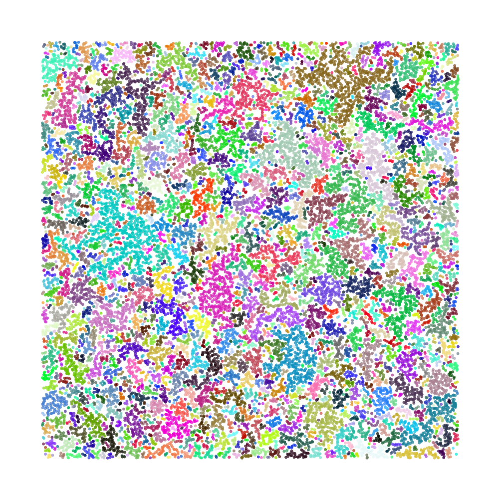
I’ll be a bit more explicit: a dot is drawn at a random location; if it does not overlap any previous dots, it gets a new color. Otherwise, the dot takes the color of the component it touches. Sometimes a new dot connects many components, and in this case, the new component takes on the color of the largest among the old components.

There’s a lot of neat questions to be asked about such a process: for instance, after drawing n dots, how many components should we expect to see? As you can see in the movie, when you draw only a few dots, most of those dots are isolated and have their own color; but after drawing a ridiculously large number of dots, they are all connected and the same color. And inbetween, something more interesting happens.

Here’s an example of “something more interesting” taken from a larger picture than the above movie:

In this fun paper [1] it is pointed out that

• homology is a very basic invariant, and
• closed manifolds are very basic objects

and so a very basic question is: what sequences of abelian groups are the homology groups of a closed simply connected manifold?

It isn’t very hard to realize any sequence of abelian groups up to the middle dimension, but that middle dimension is tricky (e.g., classify -connected -manifolds).

Anyway, I was wondering: is this realization question solvable for homology with coefficients in or ?

I’m again applying Granger causality to time series data from Intrade. This time, however, I connect box A to box B with a

• green arrow if A becoming more likely causes B to become more likely, and with a
• red arrow if A becoming more likely causes B to become less likely.

Shorter arrows suggest stronger relationships (technically, a lower p-value).

Running the algorithm on the market data since January 1, 2008 with a lag of two days produces the following graph:

And so, we see that the market data is encoding some

• tautologies (McCain’s nomination makes him more likely to be president, and McCain’s being president makes it more likely that a Republican is president) but also some
• conventional wisdom (a recession makes Clinton more likely to be nominated, but Obama less likely to be nominated; perhaps the perception that Obama would fare better in the general election explains the red arrows from “Democrat President” to Clinton, and the green arrows from “Democrat President” to Obama).

It’s amazing to me (and hopefully also to you) that the relationships between the prices of these Intrade contracts manages to encode popular sentiments.

Granger causality is a technique for determining whether one time series can be used to forecast another; since the Intrade market provides time series data for political questions, we can look at whether political outcomes can be used to forecast other political outcomes.

There’s a library for the statistical package R to do the Granger test, and Intrade produces CSV market data. I fed the market data for various contracts since January 1, 2008 into R, and the output of that into GraphViz to make a nice-looking visualization; in particular, I connect to if Granger-causes with -value less than 0.05. Darker arrows have smaller -values. This is all an embarassing misuse of statistics and -values, but it is quick and easy to do, and the results are fun to see.

Here is the graph for a lag of one day (i.e., does yesterday’s value of predict today’s value of ):

Here is the graph for a lag of two days (i.e., can the two previous days of data for be used to forecast the next day of data for ):

And here is the graph for a lag of three days:

Don’t take this too seriously. And one word of warning: an arrow from to does not mean that if is more likely, then is more likely—rather, it ought to mean that past knowledge of can be used to forecast . I suppose it would be interesting to add some color for the direction of the relationship, and maybe I’ll do that when I have another free hour.

I made some movies of some of my favorite complexes: let be the -dimensional cube, and let be the edges around the origin, and let be the square face containing the edges and . Define a subcomplex consisting of the squares and all the squares in parallel to these. It turns out that is a surface with a lot of symmetries.

In particular is a torus in , and here is a movie of it spinning:

Drew Hevle raises a very interesting question: suppose you are stranded on a desert island; what books would be entirely useless in this situation?

Here are a few books that I wouldn’t want to be stranded on an island with:

• Federal Income Tax: Code and Regulations Selected Sections
• A Million Random Digits with 100,000 Normal Deviates
• Government Phone Book USA 2000
• How to Build an Igloo: And Other Snow Shelters

Do you have other ideas for awful desert island reading?